Effort control: fishing until quota is filled
Jaideep Joshi
28 October 2024
effort_control_stock.Rmd
params_file = here::here("params/cod_params.ini")
params_file_fleet = here::here("params/fleet_1_params.ini")
Initialize a population
To simulate a fished population, we start with creating a fish and constructing a population from it, as usual.
fish = new(Fish, params_file)

pop = new(Stock, fish)
pop$readParams(params_file, F)
## [1] 0
pop$superfish_size = 0.2e6  # Each superfish contains so many fish

pop$superfish_size
## [1] 2e+05Perform Spinup
For simulating fishing, it is important for the population to start with a realistic state distribution. Therfore, we “spin-up” the population under no-fishing conditions.
v = pop$equilibriate_without_fishing(5.61) |> matrix(nrow=200, byrow=T) |> as.data.frame() |> setNames(c("ssb", "tsb", "maturity", "nr", "dr", "nfish"))Let’s see how the population state looks after no-fishing equilibrium.
d = pop$get_state()
dist = table(d$age, d$length)

par(mfrow = c(5,1), mar=c(5,5,1,1), oma=c(1,1,1,1), cex.lab=1.5, cex.axis=1.5)
plot(v$nfish~seq(1,200,1), ylab="No. of superfish", xlab="Year", type="l", col=c("cyan3"))
plot(v$maturity~seq(1,200,1), ylab="Maturity", xlab="Year", type="l", col=c("cyan3"))
plot(I(v$nr/1e9)~seq(1,200,1), ylab="Recruitment", xlab="Year", type="l", col=c("cyan3"))
plot(v$dr~seq(1,200,1), ylab="actual/potential", xlab="Year", type="l", col=c("cyan3"))

res = simulate(0, 45, F)
matplot(cbind(v$ssb/1e9, res$summaries$SSB[1:200]/1e9), ylab="SSB (MT)", xlab="Year", col=c("cyan3", "black"), lty=1, type=c("p","l"), pch=1)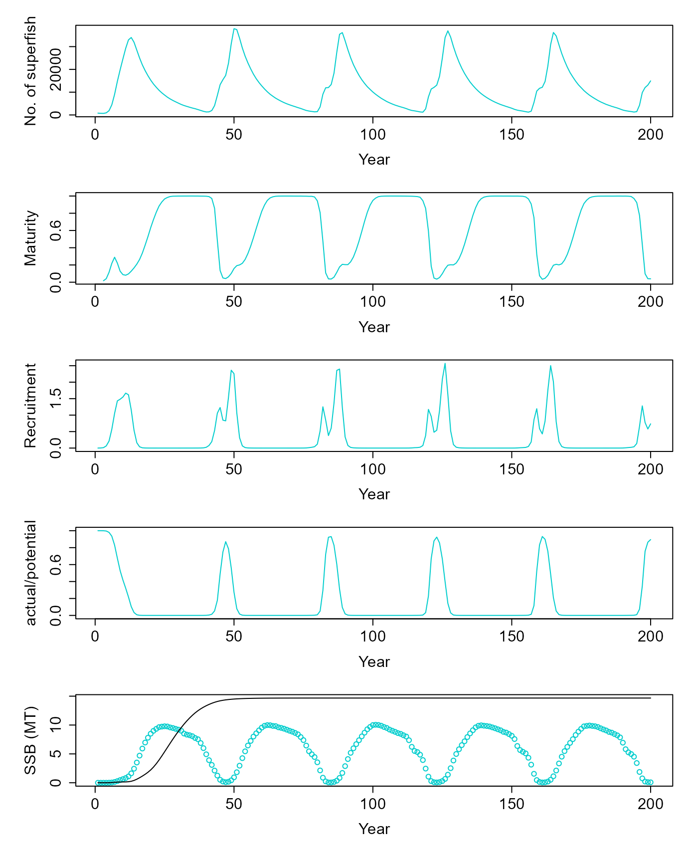
Mock fish the population to calculate fishing mortality rate (linear model)
Using the linear control model
fleet = new(Fleet)
fleet$readParams(params_file_fleet, F)
fleet$par$print()
fleet$par$control_model = "linear"
fleet$chi = 100
fleet$init_chi(pop, F_fgf, 5.61)
k_unfished = fleet$biomassFishable(pop, 0)

print(k_unfished/1e9)
## [1] 0.716761
out = fleet$harvest_dry_run(pop, quota, 5.61)

df = as.data.frame(matrix(data = out, ncol=length(progress_names), byrow = T))
colnames(df) = progress_names

print((df$B |> first())/1e9)
## [1] 0.716761
df %>%
  mutate(fish = 1:n()) %>%
  mutate(yield_err_pc = (yield-yield_expected)/yield_expected*100) %>%
  select(-B) %>%
  pivot_longer(-fish) %>%
  ggplot(aes(x=fish, y=value))+
  geom_line()+
  facet_wrap(~name, scales="free_y")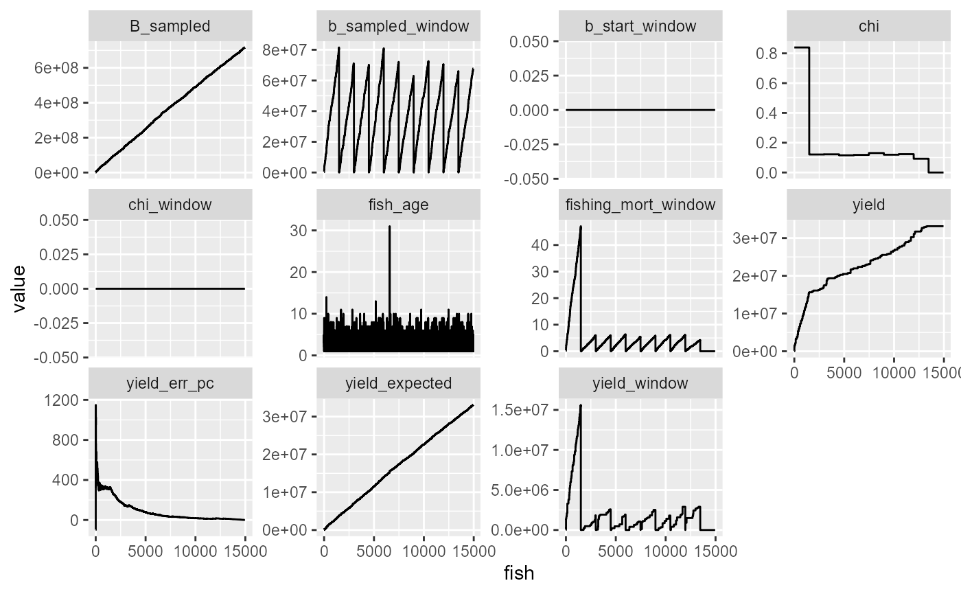
table(df$chi)##
## 1e-06 0.0922312274376576 0.115577965322125 0.118107932571342
## 1494 1496 1496 1496
## 0.119306932928501 0.120830266048479 0.121937123968437 0.123107193188716
## 1496 1496 1496 1496
## 0.1306310129756 0.839487246207361
## 1496 1495
fleet$effort_constantC(2.83e-6, 0.75, k_unfished)*fleet$par$dsea## [1] NaN
fleet$effort_constantF(2.83e-6, 0.75, k_unfished)*fleet$par$dsea## [1] 198.5158Try one more time
fleet = new(Fleet)
fleet$readParams(params_file_fleet, F)
fleet$par$print()
fleet$par$control_model = "linear"
fleet$chi = 100
fleet$init_chi(pop, F_fgf, 5.61)
k_unfished = fleet$biomassFishable(pop, 0)

out = fleet$harvest_dry_run(pop, quota, 5.61)

df = as.data.frame(matrix(data = out, ncol=length(progress_names), byrow = T))
colnames(df) = progress_names

df %>%
  mutate(fish = 1:n()) %>%
  mutate(yield_err_pc = (yield-yield_expected)/yield_expected*100) %>%
  select(-B) %>%
  pivot_longer(-fish) %>%
  ggplot(aes(x=fish, y=value))+
  geom_line()+
  facet_wrap(~name, scales="free_y")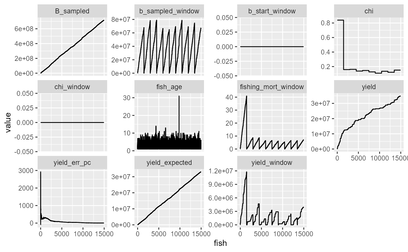
table(df$chi)##
## 0.108988683289926 0.121593809525522 0.12675069717031 0.135365859717815
## 1496 1496 1496 1496
## 0.138100867550358 0.145926182676242 0.151168257053955 0.158528391885231
## 1496 1496 1494 1496
## 0.161905724429486 0.839487246207361
## 1496 1495
fleet$effort_constantC(2.83e-6, 0.75, k_unfished)*fleet$par$dsea## [1] NaN
fleet$effort_constantF(2.83e-6, 0.75, k_unfished)*fleet$par$dsea## [1] 211.3556Mock fish the population to calculate fishing mortality rate (exp model)
Using the exponential control model
fleet = new(Fleet)
fleet$readParams(params_file_fleet, F)
fleet$par$print()
fleet$par$control_model = "exp"
fleet$chi = 100
fleet$init_chi(pop, F_fgf, 5.61)
k_unfished = fleet$biomassFishable(pop, 0)

out = fleet$harvest_dry_run(pop, quota, 5.61)

df = as.data.frame(matrix(data = out, ncol=length(progress_names), byrow = T))
colnames(df) = progress_names

df %>%
  mutate(fish = 1:n()) %>%
  mutate(yield_err_pc = (yield-yield_expected)/yield_expected*100) %>%
  select(-B) %>%
  pivot_longer(-fish) %>%
  ggplot(aes(x=fish, y=value))+
  geom_line()+
  facet_wrap(~name, scales="free_y")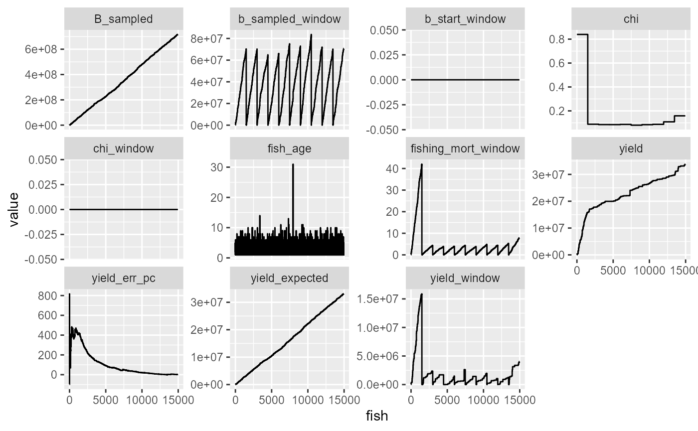
table(df$chi)##
## 0.0804539581860958 0.0846305191087766 0.0850211218025752 0.0853048816044553
## 1496 1496 1496 1496
## 0.0866759485869957 0.0874070729883764 0.0884299826940374 0.108248849284387
## 1496 1496 1496 1496
## 0.15856742590267 0.839487246207361
## 1494 1495
# df %>%
#   ggplot(aes(x=yield/k_unfished, y=catch_rate_constantF)) +
#   geom_point()+
#   geom_abline(slope=1, intercept=0, col="red")

fleet$effort_constantC(2.83e-6, 0.75, k_unfished)*fleet$par$dsea
## [1] NaN
fleet$effort_constantF(2.83e-6, 0.75, k_unfished)*fleet$par$dsea## [1] 170.9287Calculate error characteristics
pc_error = function(i, mode, h, slope){
  # quota = h*ssb_nf

  fleet = new(Fleet)
  fleet$readParams(params_file_fleet, F)
  fleet$par$control_model = mode
  fleet$par$chi0_scalar_slope = slope
  fleet$chi = 100
  fleet$init_chi(pop, F_fgf, 5.61)
  k_unfished = fleet$biomassFishable(pop, 0)

  quota = h * k_unfished

  out = fleet$harvest_dry_run(pop, quota, 5.61)

  df = as.data.frame(matrix(data = out, ncol=length(progress_names), byrow = T))
  colnames(df) = progress_names


  data.frame(
    err = df %>%
        mutate(yield_err_pc = (yield-yield_expected)/yield_expected*100) %>%
        pull(yield_err_pc) %>%
        tail(1),
    effort_c = fleet$effort_constantC(2.83e-6, 0.75, k_unfished)*fleet$par$dsea,
    effort_f = fleet$effort_constantF(2.83e-6, 0.75, k_unfished)*fleet$par$dsea
  )
}
Try exponential model
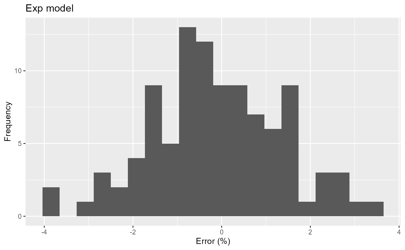
niterations = 100

res_exp = tibble(i = 1:niterations) %>%
  mutate(res = map(i, ~pc_error(.x, mode="exp", h=h, slope=0))) %>%
  unnest(res)

print(
res_exp %>%
  ggplot(aes(x=err)) +
  geom_histogram(bins=20) +
  labs(title="Exp model", x="Error (%)", y="Frequency")
)
res = expand.grid(h = seq(0.1, 0.99, length.out=10), i = 1:niterations) |>
  mutate(res = purrr::pmap(list(i, mode="exp", h, slope=0), pc_error)) |>
  unnest(res)

res |>
  ggplot(aes(x=factor(h), y=err)) +
  geom_violin() +
  stat_summary(fun=mean, geom="point", shape=23, size=2, fill="red") +
  labs(x="Harvest rate (h)", y="Error (%)", title="Error distribution (Exp model)")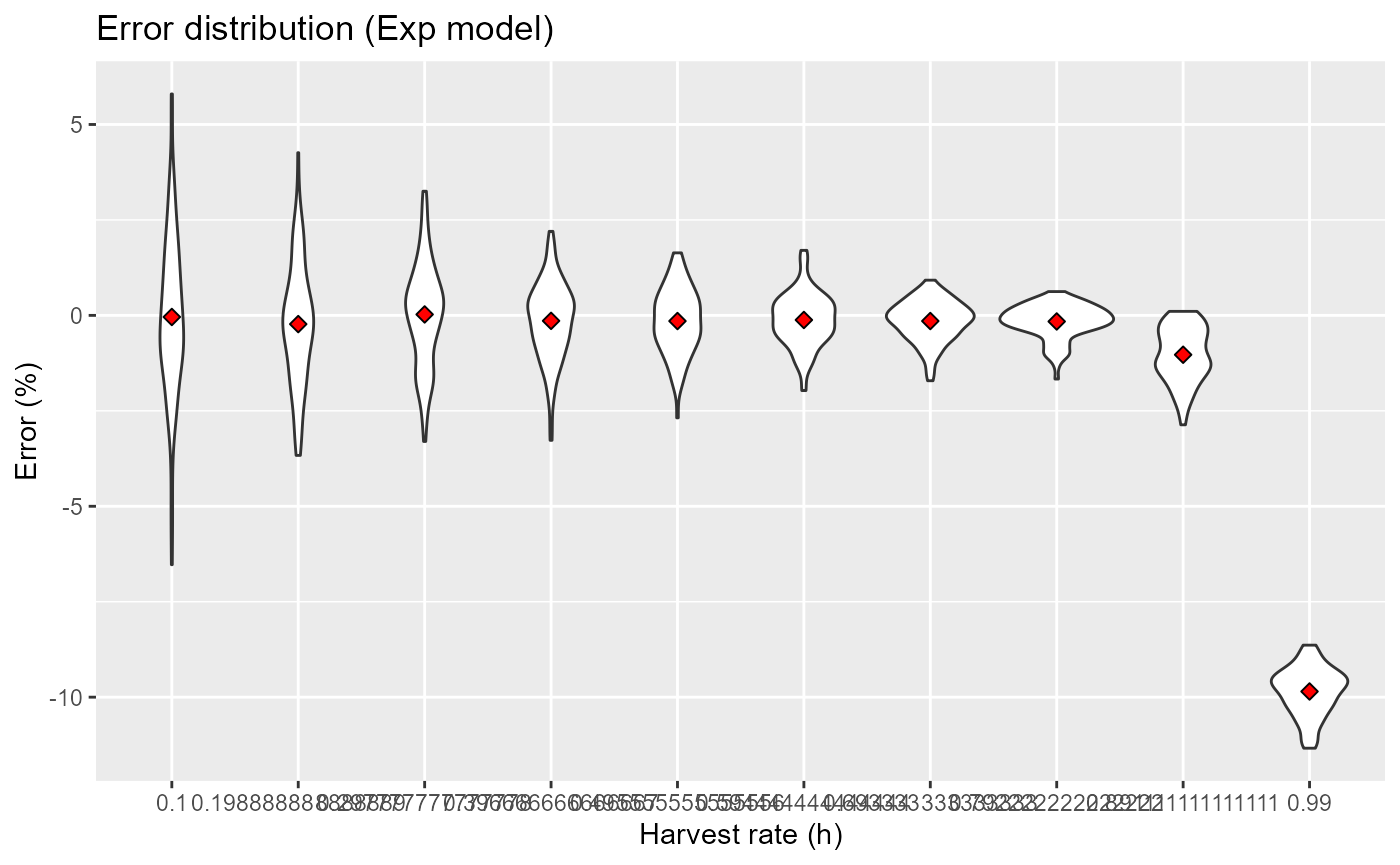
res |>
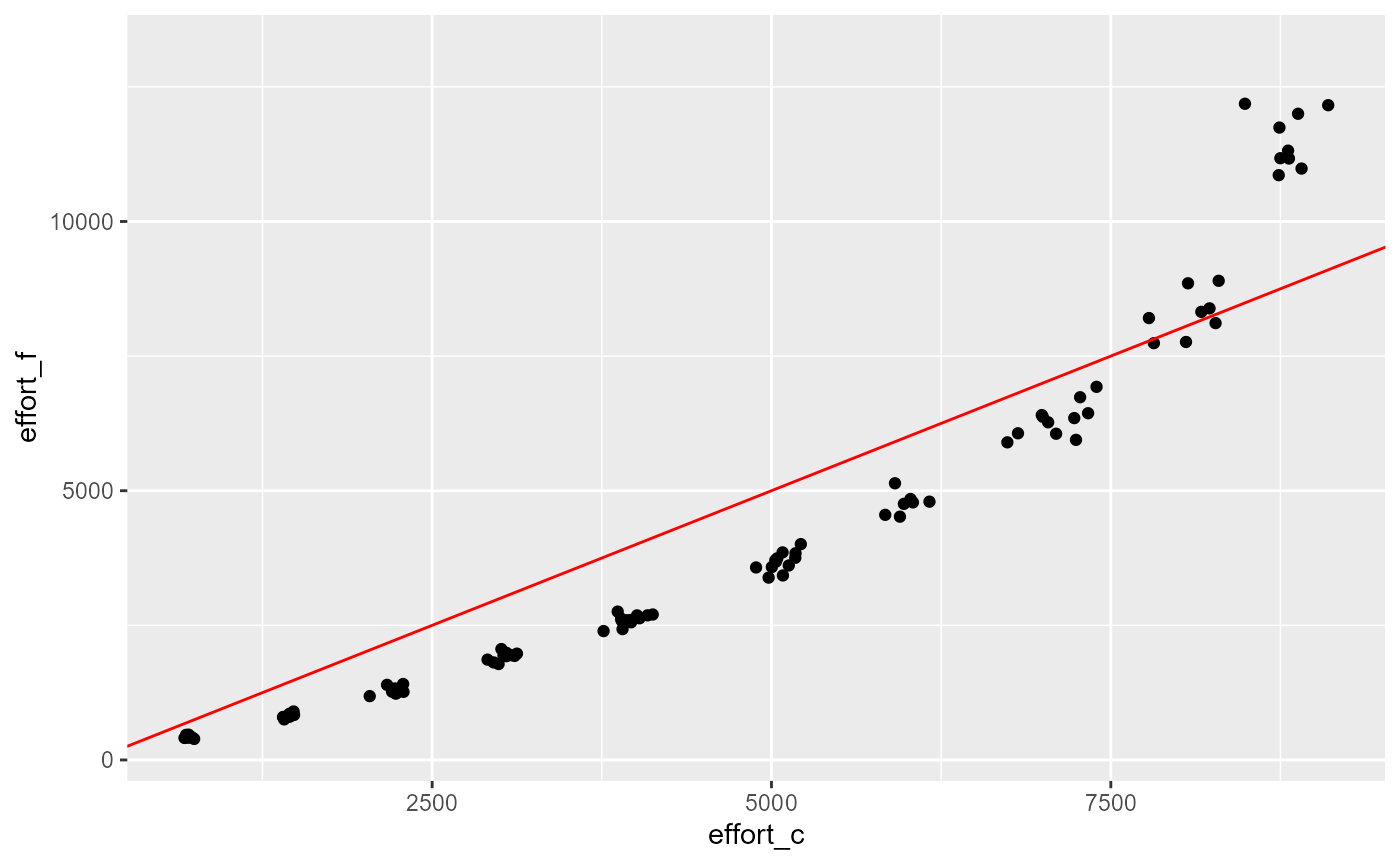
ggplot(aes(x=effort_c, y=effort_f)) +
geom_point()+
geom_abline(slope = 1, intercept = 0, col="red")## Warning: Removed 895 rows containing missing values or values outside the scale range
## (`geom_point()`).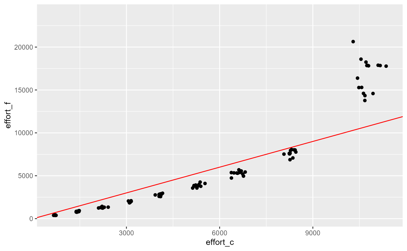
res |>
  ggplot(aes(x=effort_c, y=effort_f)) +
  geom_point()+
  geom_abline(slope = 1, intercept = 0, col="red")
## Warning: Removed 895 rows containing missing values or values outside the scale range
## (`geom_point()`).
Try linear model
res_linear = tibble(i = 1:niterations) %>%
  mutate(res = map(i, ~pc_error(.x, mode="linear", h=h, slope=0.8))) %>%
  unnest(res)

res_linear %>%
  ggplot(aes(x=err)) +
  geom_histogram(bins=20) +
  labs(title="linear model", x="Error (%)", y="Frequency")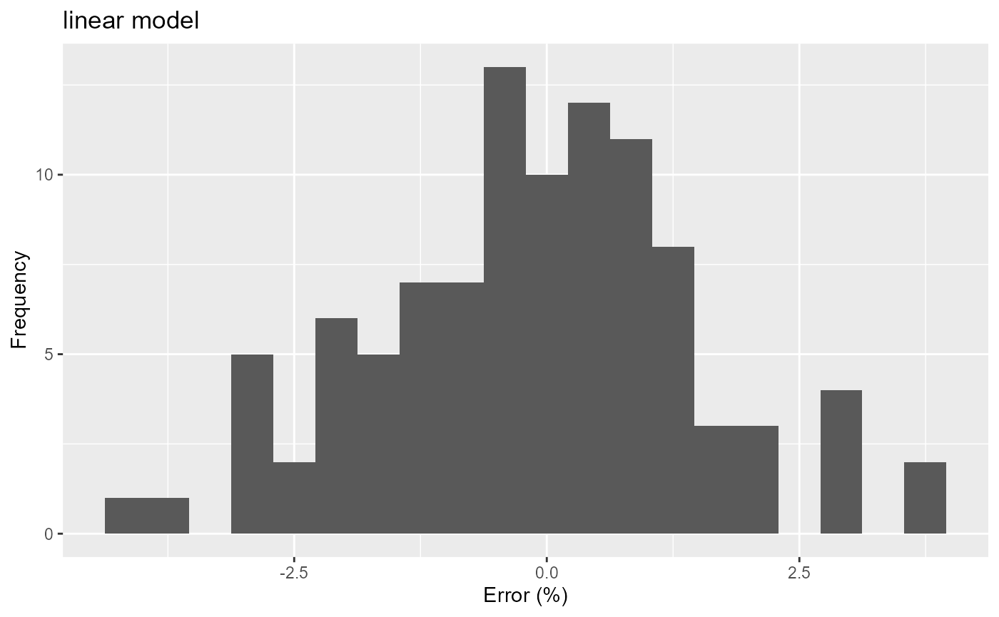
res = expand.grid(h = seq(0.1, 0.99, length.out=10), i = 1:niterations) |>
  mutate(res = purrr::pmap(list(i, mode="linear", h, slope=0.8), pc_error)) |>
  unnest(res)

res |>
  ggplot(aes(x=factor(h), y=err)) +
  geom_violin() +
  stat_summary(fun=mean, geom="point", shape=23, size=2, fill="red") +
  labs(x="Harvest rate (h)", y="Error (%)", title="Error distribution (Linear model)")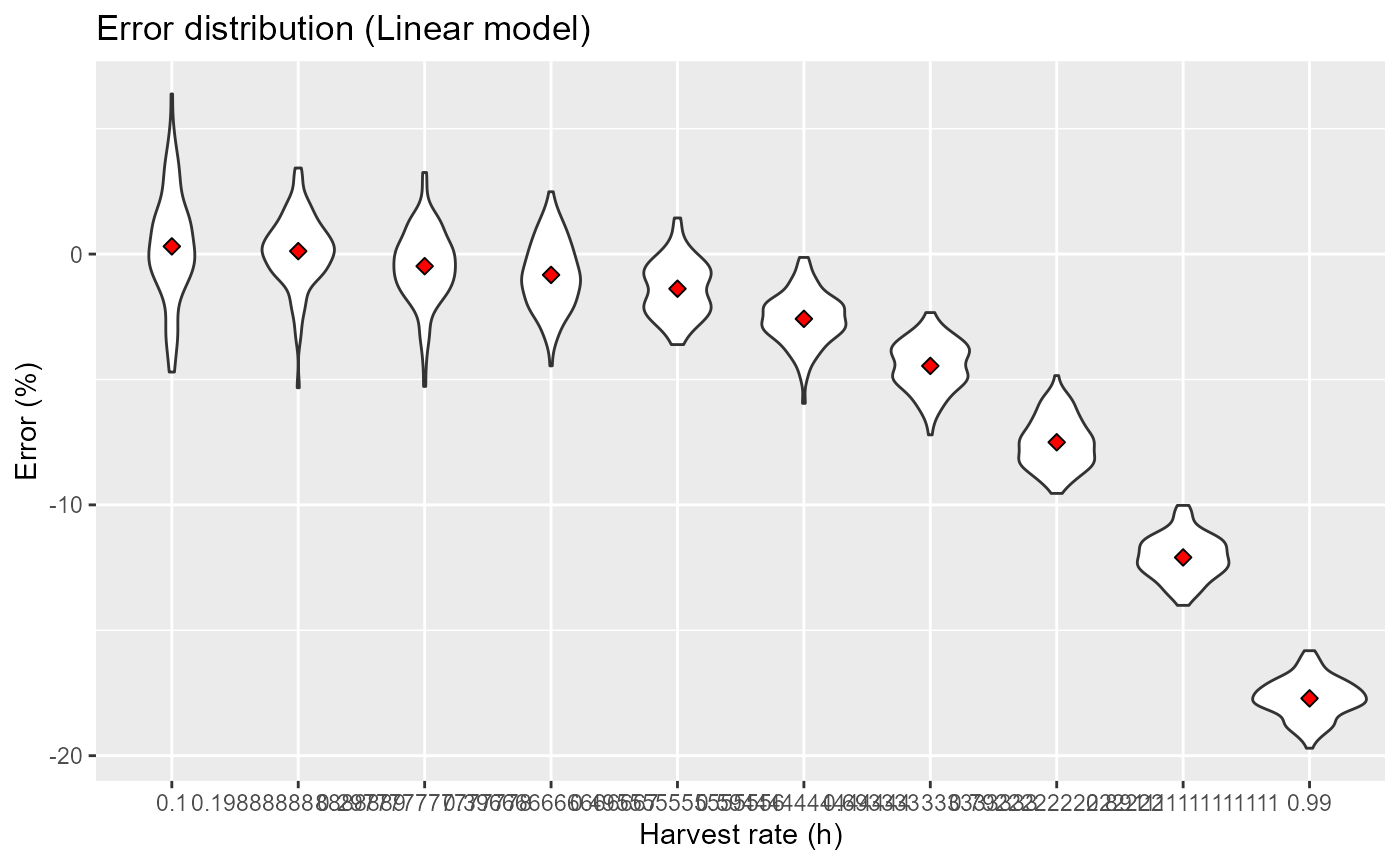
res |>
  ggplot(aes(x=effort_c, y=effort_f)) +
  geom_point()+
  geom_abline(slope = 1, intercept = 0, col="red")
## Warning: Removed 900 rows containing missing values or values outside the scale range
## (`geom_point()`).